Multi-Cycle Periodic Function Approximation using Fourier Series

Overview

In my minor FYP, I need to forecast photovoltaic (PV) power generation using Python. PV power generation is particularly interesting because it depends on the amount of solar radiation, which is not only related to the diurnal cycle but also related to the seasonal cycle. To approximate this multi-cycle periodic function, I have come up with a novel approach using the Fourier series.

In this article, I will discuss this approach, which I consider more of a clever trick than a conventional method. The trick allows for more efficient utilization of computing power. You can refer to my Chinese Graduation Thesis Excerpt, where I have applied this trick.

Fourier Series

The Fourier series is a familiar concept to engineering students, especially those studying electrical engineering students, I was one of them. The main idea of it is we can approximate a periodic function with a series of sine and cosine functions. The formula is shown below.

$$ f(t) = \frac{a_0}{2} + \sum_{n=1}^{\infty} \left( a_n \cos \left( \frac{2\pi nt}{T} \right) + b_n \sin \left( \frac{2\pi nt}{T} \right) \right) $$

where $T$ is the period of the function, $a_n$ and $b_n$ are the coefficients of the sine and cosine functions.

We can see how the Fourier series approximate a square wave with different numbers of sine and cosine functions in the picture below.

That’s awesome! Countless sine and cosine functions can approximate a periodic function that has right angles. It just bases on the previous trigonometric function and does some tiny modifications. It even reminds me of Ptolemaic model, which used deferent and epicycle to explain the motion of the planets in the geocentrism. Using lots of circular motion to approximate complex planetary motions observed from Earth is very similar to using lots of sine and cosine functions to approximate a periodic function. You can see an interesting explanation in this post.

Multi-Cycle Periodic Function

Usually, if we want to use Python to approximate a periodic function, we can use the code below to build a Fourier series.

fourier_features = np.column_stack(
[np.cos(omega * n * x) for n in range(1, num_terms + 1)] +
[np.sin(omega * n * x) for n in range(1, num_terms + 1)])

Now let’s turn back to the multi-cycle periodic function. If some variables are influenced by more than one periodic factor, for example, solar radiation. We can use the code below:

omega_y = 2 * np.pi / (365 * 24)
omega_d = 2 * np.pi / 24

fourier_features = np.column_stack(
[np.cos(omega_y * n * hours) for n in range(1, num_terms + 1)] +
[np.sin(omega_y * n * hours) for n in range(1, num_terms + 1)] +
[np.cos(omega_d * n * hours) for n in range(1, num_terms + 1)] +
[np.sin(omega_d * n * hours) for n in range(1, num_terms + 1)])

Can you see the difference? I just replaced $x$ with $hour$, declared two different angular frequencies $\omega_y$ and $\omega_d$, and added two more sine and cosine functions. It’s very simple but also efficient. The two angular frequencies correspond to the two periodic factors, the annual cycle and the diurnal cycle. You can think of it as a better allocation of computing power.

If we calculate the Fourier series built by the first code, all terms will base on one angular frequency $\omega$. But if we calculate the Fourier series built by the second code, the terms will base on two angular frequencies $\omega_y$ and $\omega_d$.

For instance, if the second code is written in the first style, and the number of terms is 100, the term having the minimum period is

$$ \cos \left( \frac{2\pi \times 100 \times hour}{365 \times 24} \right) + \sin \left( \frac{2\pi \times 100 \times hour}{365 \times 24} \right) $$

Its period is $365 \times 24 / 100 = 87.6$, which is even bigger than the $\omega_d$’s period $24$. So in the first style, even if we calculate 100 terms, we still cannot consider the diurnal cycle. But in the second style, we can consider the diurnal cycle with only 2 terms.

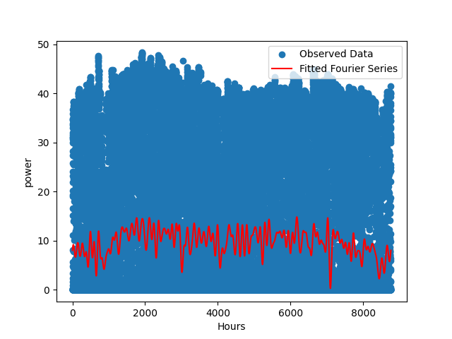
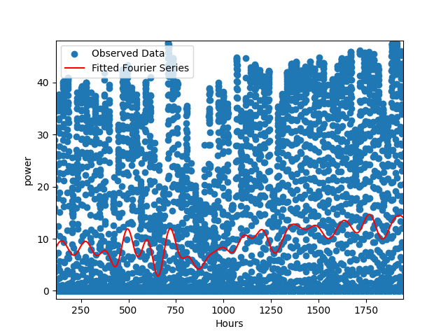
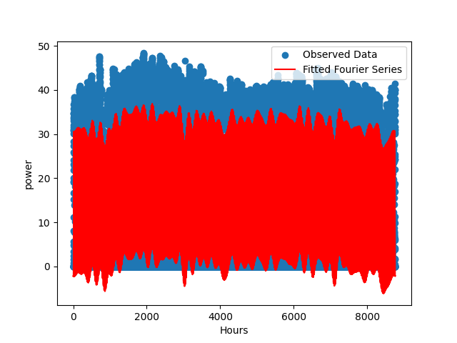
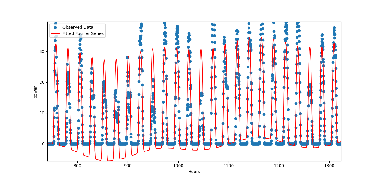
Program Output

I wrote a simple program to show the difference between the two styles. We can see with the same computing power, the second style can approximate the multi-cycle periodic function much better. In the first style the num_terms is 90, in the second style the num_terms is 45.

Output in the first style

Output in the second style